Samples, populations and sampling

Remember, the role of descriptive statistics is to concisely summarize what we do know. In contrast, the purpose of inferential statistics is to "learn what we do not know from what we do". What kinds of things would we like to learn about? And how do we learn them? These are the questions that lie at the heart of inferential statistics, and they are traditionally divided into two "big ideas": estimation and hypothesis testing. The goal in this chapter is to introduce the first of these big ideas, estimation theory, but we'll talk about sampling theory first because estimation theory doesn't make sense until you understand sampling. So, this chapter divides into sampling theory, and how to make use of sampling theory to discuss how statisticians think about estimation. We have already done lots of sampling, so you are already familiar with some of the big ideas.

Sampling theory plays a huge role in specifying the assumptions upon which your statistical inferences rely. And in order to talk about "making inferences" the way statisticians think about it, we need to be a bit more explicit about what it is that we're drawing inferences from (the sample) and what it is that we're drawing inferences about (the population).

In almost every situation of interest, what we have available to us as researchers is a sample of data. We might have run experiment with some number of participants; a polling company might have phoned some number of people to ask questions about voting intentions; etc. Regardless: the data set available to us is finite, and incomplete. We can't possibly get every person in the world to do our experiment; a polling company doesn't have the time or the money to ring up every voter in the country etc. In our earlier discussion of descriptive statistics, this sample was the only thing we were interested in. Our only goal was to find ways of describing, summarizing and graphing that sample. This is about to change.

Defining a population

A sample is a concrete thing. You can open up a data file, and there's the data from your sample. A population, on the other hand, is a more abstract idea. It refers to the set of all possible people, or all possible observations, that you want to draw conclusions about, and is generally much bigger than the sample. In an ideal world, the researcher would begin the study with a clear idea of what the population of interest is, since the process of designing a study and testing hypotheses about the data that it produces does depend on the population about which you want to make statements. However, that doesn't always happen in practice: usually the researcher has a fairly vague idea of what the population is and designs the study as best he/she can on that basis.

Sometimes it's easy to state the population of interest. For instance, in the "polling company" example, the population consisted of all voters enrolled at the a time of the study – millions of people. The sample was a set of 1000 people who all belong to that population. In most situations the situation is much less simple. In a typical a psychological experiment, determining the population of interest is a bit more complicated. Suppose I run an experiment using 100 undergraduate students as my participants. My goal, as a cognitive scientist, is to try to learn something about how the mind works. So, which of the following would count as "the population":

• All of the undergraduate psychology students at the University of Adelaide?

• Undergraduate psychology students in general, anywhere in the world?

• Australians currently living?

• Australians of similar ages to my sample?

• Anyone currently alive?

• Any human being, past, present or future?

• Any biological organism with a sufficient degree of intelligence operating in a terrestrial environment?

• Any intelligent being?

Each of these defines a real group of mind-possessing entities, all of which might be of interest to me as a cognitive scientist, and it's not at all clear which one ought to be the true population of interest.

Simple random samples

Irrespective of how we define the population, the critical point is that the sample is a subset of the population, and our goal is to use our knowledge of the sample to draw inferences about the properties of the population. The relationship between the two depends on the procedure by which the sample was selected. This procedure is referred to as a sampling method, and it is important to understand why it matters.

To keep things simple, imagine we have a bag containing 10 chips. Each chip has a unique letter printed on it, so we can distinguish between the 10 chips. The chips come in two colors, black and white.

This set of chips is the population of interest, and it is depicted graphically on the left of Figure \@ref(fig:srs1).

As you can see from looking at the picture, there are 4 black chips and 6 white chips, but of course in real life we wouldn't know that unless we looked in the bag. Now imagine you run the following "experiment": you shake up the bag, close your eyes, and pull out 4 chips without putting any of them back into the bag. First out comes the $a$ chip (black), then the $c$ chip (white), then $j$ (white) and then finally $b$ (black). If you wanted, you could then put all the chips back in the bag and repeat the experiment, as depicted on the right hand side of Figure\@ref(fig:srs1). Each time you get different results, but the procedure is identical in each case. The fact that the same procedure can lead to different results each time, we refer to it as a random process. However, because we shook the bag before pulling any chips out, it seems reasonable to think that every chip has the same chance of being selected. A procedure in which every member of the population has the same chance of being selected is called a simple random sample. The fact that we did not put the chips back in the bag after pulling them out means that you can't observe the same thing twice, and in such cases the observations are said to have been sampled without replacement.

To help make sure you understand the importance of the sampling procedure, consider an alternative way in which the experiment could have been run. Suppose that my 5-year old son had opened the bag, and decided to pull out four black chips without putting any of them back in the bag. This biased sampling scheme is depicted in Figure \@ref(fig:brs).

Now consider the evidentiary value of seeing 4 black chips and 0 white chips. Clearly, it depends on the sampling scheme, does it not? If you know that the sampling scheme is biased to select only black chips, then a sample that consists of only black chips doesn't tell you very much about the population! For this reason, statisticians really like it when a data set can be considered a simple random sample, because it makes the data analysis much easier.

A third procedure is worth mentioning. This time around we close our eyes, shake the bag, and pull out a chip. This time, however, we record the observation and then put the chip back in the bag. Again we close our eyes, shake the bag, and pull out a chip. We then repeat this procedure until we have 4 chips. Data sets generated in this way are still simple random samples, but because we put the chips back in the bag immediately after drawing them it is referred to as a sample with replacement. The difference between this situation and the first one is that it is possible to observe the same population member multiple times, as illustrated in Figure \@ref(fig:srs2).

Most psychology experiments tend to be sampling without replacement, because the same person is not allowed to participate in the experiment twice. However, most statistical theory is based on the assumption that the data arise from a simple random sample with replacement. In real life, this very rarely matters. If the population of interest is large (e.g., has more than 10 entities!) the difference between sampling with- and without- replacement is too small to be concerned with. The difference between simple random samples and biased samples, on the other hand, is not such an easy thing to dismiss.

Most samples are not simple random samples

As you can see from looking at the list of possible populations that I showed above, it is almost impossible to obtain a simple random sample from most populations of interest. When I run experiments, I'd consider it a minor miracle if my participants turned out to be a random sampling of the undergraduate psychology students at Adelaide university, even though this is by far the narrowest population that I might want to generalize to. A thorough discussion of other types of sampling schemes is beyond the scope of this book, but to give you a sense of what's out there I'll list a few of the more important ones:

• Stratified sampling. Suppose your population is (or can be) divided into several different sub-populations, or strata. Perhaps you're running a study at several different sites, for example. Instead of trying to sample randomly from the population as a whole, you instead try to collect a separate random sample from each of the strata. Stratified sampling is sometimes easier to do than simple random sampling, especially when the population is already divided into the distinct strata. It can also be more efficient that simple random sampling, especially when some of the sub-populations are rare. For instance, when studying schizophrenia it would be much better to divide the population into two strata (schizophrenic and not-schizophrenic), and then sample an equal number of people from each group. If you selected people randomly, you would get so few schizophrenic people in the sample that your study would be useless. This specific kind of of stratified sampling is referred to as oversampling because it makes a deliberate attempt to over-represent rare groups.

• Snowball sampling is a technique that is especially useful when sampling from a "hidden" or hard to access population, and is especially common in social sciences. For instance, suppose the researchers want to conduct an opinion poll among transgender people. The research team might only have contact details for a few trans folks, so the survey starts by asking them to participate (stage 1). At the end of the survey, the participants are asked to provide contact details for other people who might want to participate. In stage 2, those new contacts are surveyed. The process continues until the researchers have sufficient data. The big advantage to snowball sampling is that it gets you data in situations that might otherwise be impossible to get any. On the statistical side, the main disadvantage is that the sample is highly non-random, and non-random in ways that are difficult to address. On the real life side, the disadvantage is that the procedure can be unethical if not handled well, because hidden populations are often hidden for a reason. I chose transgender people as an example here to highlight this: if you weren't careful you might end up outing people who don't want to be outed (very, very bad form), and even if you don't make that mistake it can still be intrusive to use people's social networks to study them. It's certainly very hard to get people's informed consent before contacting them, yet in many cases the simple act of contacting them and saying "hey we want to study you" can be hurtful. Social networks are complex things, and just because you can use them to get data doesn't always mean you should.

• Convenience sampling is more or less what it sounds like. The samples are chosen in a way that is convenient to the researcher, and not selected at random from the population of interest. Snowball sampling is one type of convenience sampling, but there are many others. A common example in psychology are studies that rely on undergraduate psychology students. These samples are generally non-random in two respects: firstly, reliance on undergraduate psychology students automatically means that your data are restricted to a single sub-population. Secondly, the students usually get to pick which studies they participate in, so the sample is a self selected subset of psychology students not a randomly selected subset. In real life, most studies are convenience samples of one form or another. This is sometimes a severe limitation, but not always.

How much does it matter if you don't have a simple random sample?

Okay, so real world data collection tends not to involve nice simple random samples. Does that matter? A little thought should make it clear to you that it can matter if your data are not a simple random sample: just think about the difference between Figures \@ref(fig:srs1) and \@ref(fig:brs). However, it's not quite as bad as it sounds. Some types of biased samples are entirely unproblematic. For instance, when using a stratified sampling technique you actually know what the bias is because you created it deliberately, often to increase the effectiveness of your study, and there are statistical techniques that you can use to adjust for the biases you've introduced (not covered in this book!). So in those situations it's not a problem.

More generally though, it's important to remember that random sampling is a means to an end, not the end in itself. Let's assume you've relied on a convenience sample, and as such you can assume it's biased. A bias in your sampling method is only a problem if it causes you to draw the wrong conclusions. When viewed from that perspective, I'd argue that we don't need the sample to be randomly generated in every respect: we only need it to be random with respect to the psychologically-relevant phenomenon of interest. Suppose I'm doing a study looking at working memory capacity. In study 1, I actually have the ability to sample randomly from all human beings currently alive, with one exception: I can only sample people born on a Monday. In study 2, I am able to sample randomly from the Australian population. I want to generalize my results to the population of all living humans. Which study is better? The answer, obviously, is study 1. Why? Because we have no reason to think that being "born on a Monday" has any interesting relationship to working memory capacity. In contrast, I can think of several reasons why "being Australian" might matter. Australia is a wealthy, industrialized country with a very well-developed education system. People growing up in that system will have had life experiences much more similar to the experiences of the people who designed the tests for working memory capacity. This shared experience might easily translate into similar beliefs about how to "take a test", a shared assumption about how psychological experimentation works, and so on. These things might actually matter. For instance, "test taking" style might have taught the Australian participants how to direct their attention exclusively on fairly abstract test materials relative to people that haven't grown up in a similar environment; leading to a misleading picture of what working memory capacity is.

There are two points hidden in this discussion. Firstly, when designing your own studies, it's important to think about what population you care about, and try hard to sample in a way that is appropriate to that population. In practice, you're usually forced to put up with a "sample of convenience" (e.g., psychology lecturers sample psychology students because that's the least expensive way to collect data, and our coffers aren't exactly overflowing with gold), but if so you should at least spend some time thinking about what the dangers of this practice might be.

Secondly, if you're going to criticize someone else's study because they've used a sample of convenience rather than laboriously sampling randomly from the entire human population, at least have the courtesy to offer a specific theory as to how this might have distorted the results. Remember, everyone in science is aware of this issue, and does what they can to alleviate it. Merely pointing out that "the study only included people from group BLAH" is entirely unhelpful, and borders on being insulting to the researchers, who are aware of the issue. They just don't happen to be in possession of the infinite supply of time and money required to construct the perfect sample. In short, if you want to offer a responsible critique of the sampling process, then be helpful. Rehashing the blindingly obvious truisms that I've been rambling on about in this section isn't helpful.

Population parameters and sample statistics

Okay. Setting aside the thorny methodological issues associated with obtaining a random sample, let's consider a slightly different issue. Up to this point we have been talking about populations the way a scientist might. To a psychologist, a population might be a group of people. To an ecologist, a population might be a group of bears. In most cases the populations that scientists care about are concrete things that actually exist in the real world.

Statisticians, however, are a funny lot. On the one hand, they are interested in real world data and real science in the same way that scientists are. On the other hand, they also operate in the realm of pure abstraction in the way that mathematicians do. As a consequence, statistical theory tends to be a bit abstract in how a population is defined. In much the same way that psychological researchers operationalize our abstract theoretical ideas in terms of concrete measurements, statisticians operationalize the concept of a "population" in terms of mathematical objects that they know how to work with. You've already come across these objects they're called probability distributions (remember, the place where data comes from).

The idea is quite simple. Let's say we're talking about IQ scores. To a psychologist, the population of interest is a group of actual humans who have IQ scores. A statistician "simplifies" this by operationally defining the population as the probability distribution depicted in Figure \@ref(fig:IQdist)a.

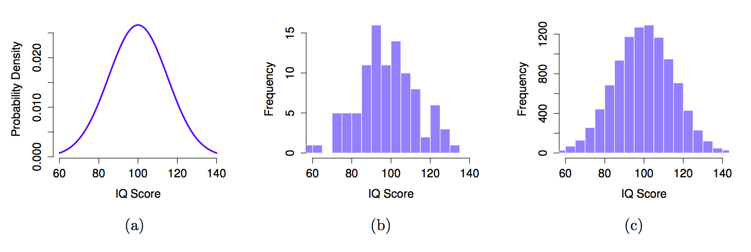
IQ tests are designed so that the average IQ is 100, the standard deviation of IQ scores is 15, and the distribution of IQ scores is normal. These values are referred to as the population parameters because they are characteristics of the entire population. That is, we say that the population mean $\mu$ is 100, and the population standard deviation $\sigma$ is 15.

Now suppose we collect some data. We select 100 people at random and administer an IQ test, giving a simple random sample from the population. The sample would consist of a collection of numbers like this:

106 101 98 80 74 ... 107 72 100

Each of these IQ scores is sampled from a normal distribution with mean 100 and standard deviation 15. So if I plot a histogram of the sample, I get something like the one shown in Figure \@ref(fig:IQdist)b. As you can see, the histogram is roughly the right shape, but it's a very crude approximation to the true population distribution shown in Figure \@ref(fig:IQdist)a. The mean of the sample is fairly close to the population mean 100 but not identical. In this case, it turns out that the people in the sample have a mean IQ of 98.5, and the standard deviation of their IQ scores is 15.9. These sample statistics are properties of the data set, and although they are fairly similar to the true population values, they are not the same. In general, sample statistics are the things you can calculate from your data set, and the population parameters are the things you want to learn about. Later on in this chapter we'll talk about how you can estimate population parameters using your sample statistics and how to work out how confident you are in your estimates but before we get to that there's a few more ideas in sampling theory that you need to know about.

The law of large numbers

We just looked at the results of one fictitious IQ experiment with a sample size of $N=100$. The results were somewhat encouraging: the true population mean is 100, and the sample mean of 98.5 is a pretty reasonable approximation to it. In many scientific studies that level of precision is perfectly acceptable, but in other situations you need to be a lot more precise. If we want our sample statistics to be much closer to the population parameters, what can we do about it?

The obvious answer is to collect more data. Suppose that we ran a much larger experiment, this time measuring the IQ's of 10,000 people. We can simulate the results of this experiment using R, using the rnorm() function, which generates random numbers sampled from a normal distribution. For an experiment with a sample size of n = 10000, and a population with mean = 100 and sd = 15, R produces our fake IQ data using these commands:

Cool, we just generated 10,000 fake IQ scores. Where did they go? Well, they went into the variable IQ on my computer. You can do the same on your computer too by copying the above code. 10,000 numbers is too many numbers to look at. We can look at the first 100 like this:

We can compute the mean IQ using the command np.mean(IQ) and the standard deviation using the command np.std(IQ), and draw a histogram using plt.hist().

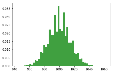
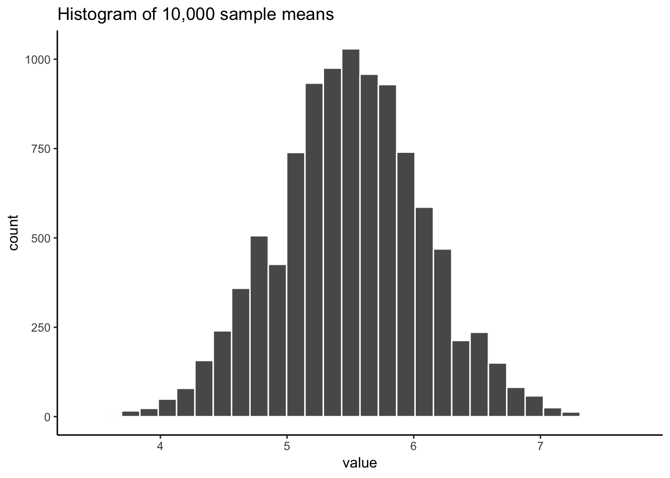
The histogram of this much larger sample is shown in Figure above. Even a moment's inspections makes clear that the larger sample is a much better approximation to the true population distribution than the smaller one. This is reflected in the sample statistics: the mean IQ for the larger sample turns out to be 99.9, and the standard deviation is 15.1. These values are now very close to the true population.

I feel a bit silly saying this, but the thing I want you to take away from this is that large samples generally give you better information. I feel silly saying it because it's so bloody obvious that it shouldn't need to be said. In fact, it's such an obvious point that when Jacob Bernoulli – one of the founders of probability theory – formalized this idea back in 1713, he was kind of a jerk about it. Here's how he described the fact that we all share this intuition:

For even the most stupid of men, by some instinct of nature, by himself and without any instruction (which is a remarkable thing), is convinced that the more observations have been made, the less danger there is of wandering from one's goal (see Stigler, 1986, p65).

Okay, so the passage comes across as a bit condescending (not to mention sexist), but his main point is correct: it really does feel obvious that more data will give you better answers. The question is, why is this so? Not surprisingly, this intuition that we all share turns out to be correct, and statisticians refer to it as the law of large numbers. The law of large numbers is a mathematical law that applies to many different sample statistics, but the simplest way to think about it is as a law about averages. The sample mean is the most obvious example of a statistic that relies on averaging (because that's what the mean is... an average), so let's look at that. When applied to the sample mean, what the law of large numbers states is that as the sample gets larger, the sample mean tends to get closer to the true population mean. Or, to say it a little bit more precisely, as the sample size "approaches" infinity (written as $N \rightarrow \infty$) the sample mean approaches the population mean ($\bar{X} \rightarrow \mu$).

I don't intend to subject you to a proof that the law of large numbers is true, but it's one of the most important tools for statistical theory. The law of large numbers is the thing we can use to justify our belief that collecting more and more data will eventually lead us to the truth. For any particular data set, the sample statistics that we calculate from it will be wrong, but the law of large numbers tells us that if we keep collecting more data those sample statistics will tend to get closer and closer to the true population parameters.

Sampling distributions and the central limit theorem

The law of large numbers is a very powerful tool, but it's not going to be good enough to answer all our questions. Among other things, all it gives us is a "long run guarantee". In the long run, if we were somehow able to collect an infinite amount of data, then the law of large numbers guarantees that our sample statistics will be correct. But as John Maynard Keynes famously argued in economics, a long run guarantee is of little use in real life:

[The] long run is a misleading guide to current affairs. In the long run we are all dead. Economists set themselves too easy, too useless a task, if in tempestuous seasons they can only tell us, that when the storm is long past, the ocean is flat again. @Keynes1923 [p. 80]

As in economics, so too in psychology and statistics. It is not enough to know that we will eventually arrive at the right answer when calculating the sample mean. Knowing that an infinitely large data set will tell me the exact value of the population mean is cold comfort when my actual data set has a sample size of $N=100$. In real life, then, we must know something about the behavior of the sample mean when it is calculated from a more modest data set!

Sampling distribution of the sample means

"Oh no, what is the sample distribution of the sample means? Is that even allowed in English?". Yes, unfortunately, this is allowed. The sampling distribution of the sample means is the next most important thing you will need to understand. IT IS SO IMPORTANT THAT IT IS NECESSARY TO USE ALL CAPS. It is only confusing at first because it's long and uses sampling and sample in the same phrase.

Don't worry, we've been prepping you for this. You know what a distribution is right? It's where numbers comes from. It makes some numbers occur more or less frequently, or the same as other numbers. You know what a sample is right? It's the numbers we take from a distribution. So, what could the sampling distribution of the sample means refer to?

First, what do you think the sample means refers to? Well, if you took a sample of numbers, you would have a bunch of numbers...then, you could compute the mean of those numbers. The sample mean is the mean of the numbers in the sample. That is all. So, what is this distribution you speak of? Well, what if you took a bunch of samples, put one here, put one there, put some other ones other places. You have a lot of different samples of numbers. You could compute the mean for each them. Then you would have a bunch of means. What do those means look like? Well, if you put them in a histogram, you could find out. If you did that, you would be looking at (roughly) a distribution, AKA the sampling distribution of the sample means.

"I'm following along sort of, why would I want to do this instead of watching Netflix...". Because, the sampling distribution of the sample means gives you another window into chance. A very useful one that you can control, just like your remote control, by pressing the right design buttons.

Seeing the pieces

To make a sampling distribution of the sample means, we just need the following:

1. A distribution to take numbers from
2. A bunch of different samples from the distribution
3. The means of each of the samples
4. Get all of the sample means, and plot them in a histogram

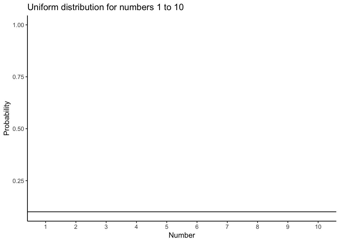
Let's do those four things. We will sample numbers from the uniform distribution, it looks like this if we are sampling from the set of integers from 1 to 10:

OK, now let's take a bunch of samples from that distribution. We will set our sample-size to 20. It's easier to see how the sample mean behaves in a movie. Each histogram shows a new sample. The red line shows where the mean of the sample is. The samples are all very different from each other, but the red line doesn't move around very much, it always stays near the middle. However, the red line does move around a little bit, and this variance is what we call the sampling distribution of the sample mean.

OK, what have we got here? We have an animiation of 10 different samples. Each sample has 20 observations and these are summarized in each of histograms that show up in the animiation. Each histogram has a red line. The red line shows you where the mean of each sample is located. So, we have found the sample means for the 10 different samples from a uniform distribution.

First question. Are the sample means all the same? The answer is no. They are all kind of similar to each other though, they are all around five plus or minus a few numbers. This is interesting. Although all of our samples look pretty different from one another, the means of our samples look more similar than different.

Second question. What should we do with the means of our samples? Well, how about we collect them them all, and then plot a histogram of them. This would allow us to see what the distribution of the sample means looks like. The next histogram is just this. Except, rather than taking 10 samples, we will take 10,000 samples. For each of them we will compute the means. So, we will have 10,000 means. This is the histogram of the sample means:

"Wait what? This doesn't look right. I thought we were taking samples from a uniform distribution. Uniform distributions are flat. THIS DOES NOT LOOK LIKE A FLAT DISTRIBTUION, WHAT IS GOING ON, AAAAAGGGHH.". We feel your pain.

Remember, we are looking at the distribution of sample means. It is indeed true that the distribution of sample means does not look the same as the distribution we took the samples from. Our distribution of sample means goes up and down. In fact, this will almost always be the case for distributions of sample means. This fact is called the central limit theorem, which we talk about later.

For now, let's talk about about what's happening. Remember, we have been sampling numbers between the range 1 to 10. We are supposed to get each number with roughly equal frequency, because we are sampling from a uniform distribution. So, let's say we took a sample of 10 numbers, and happened to get one of each from 1 to 10.

1 2 3 4 5 6 7 8 9 10

What is the mean of those numbers? Well, its 1+2+3+4+5+6+7+8+9+10 = 55 / 10 = 5.5. Imagine if we took a bigger sample, say of 20 numbers, and again we got exactly 2 of each number. What would the mean be? It would be (1+2+3+4+5+6+7+8+9+10)*2 = 110 / 20 = 5.5. Still 5.5. You can see here, that the mean value of our uniform distribution is 5.5. Now that we know this, we might expect that most of our samples will have a mean near this number. We already know that every sample won't be perfect, and it won't have exactly an equal amount of every number. So, we will expect the mean of our samples to vary a little bit. The histogram that we made shows the variation. Not surprisingly, the numbers vary around the value 5.5.

Sampling distributions exist for any sample statistic!

One thing to keep in mind when thinking about sampling distributions is that any sample statistic you might care to calculate has a sampling distribution. For example, suppose that each time you sampled some numbers from an experiment you wrote down the largest number in the experiment. Doing this over and over again would give you a very different sampling distribution, namely the sampling distribution of the maximum. You could calculate the smallest number, or the mode, or the median, of the variance, or the standard deviation, or anything else from your sample. Then, you could repeat many times, and produce the sampling distribution of those statistics. Neat!

Just for fun here are some different sampling distributions for different statistics. We will take a normal distribution with mean = 100, and standard deviation =20. Then, we'll take lots of samples with n = 50 (50 observations per sample). We'll save all of the sample statistics, then plot their histograms. Let's do it:

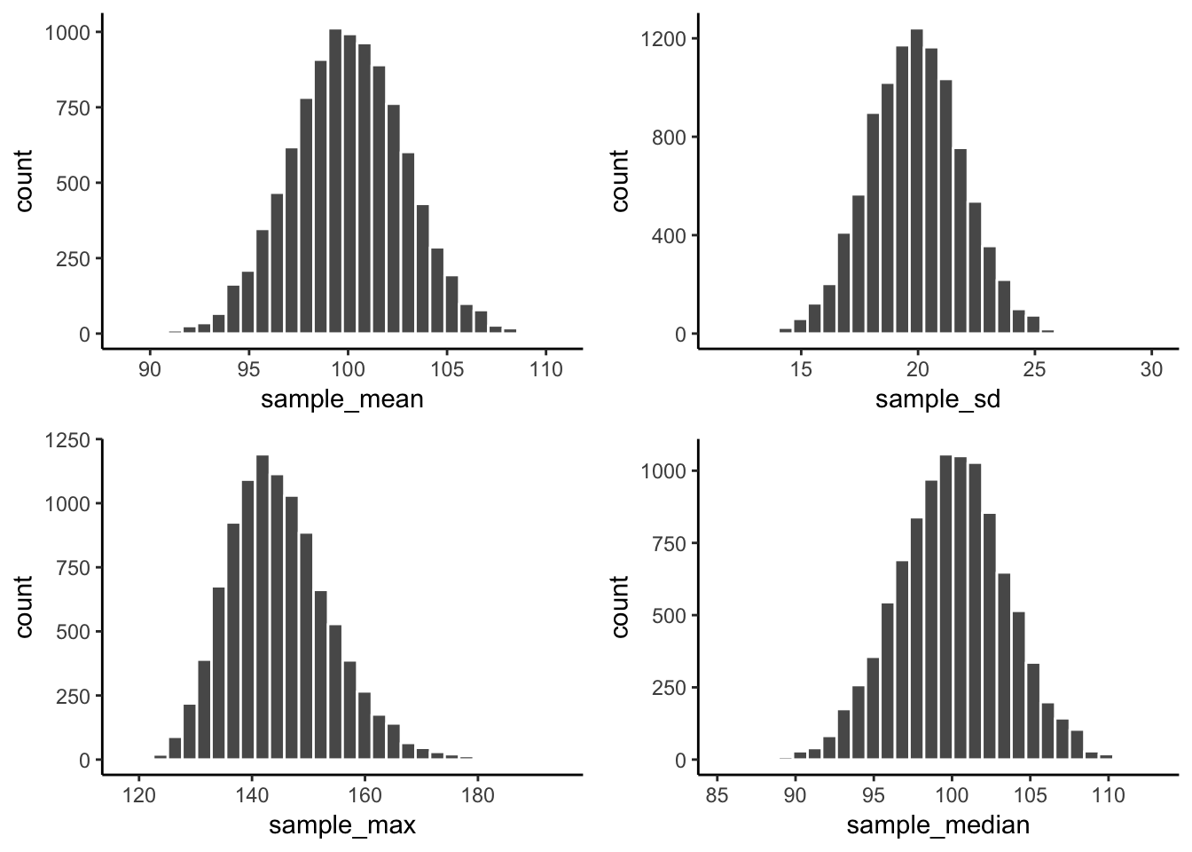
We just computed 4 different sampling distributions, for the mean, standard deviation, maximum value, and the median. If you just look quickly at these histograms you might think they all basically look the same. Hold up now. It's very important to look at the x-axes. They are different. For example, the sample mean goes from about 90 to 110, whereas the standard deviation goes from 15 to 25.

These sampling distributions are super important, and worth thinking about. What should you think about? Well, here's a clue. These distributions are telling you what to expect from your sample. Critically, they are telling you what you should expect from a sample, when you take one from the specific distribution that we used (normal distribution with mean =100 and SD = 20). What have we learned. We've learned a tonne. We've learned that we can expect our sample to have a mean somewhere between 90 and 108ish. Notice, the sample means are never more extreme. We've learned that our sample will usually have some variance, and that the the standard deviation will be somewhere between 15 and 25 (never much more extreme than that). We can see that sometime we get some big numbers, say between 120 and 180, but not much bigger than that. And, we can see that the median is pretty similar to the mean. If you ever took a sample of 50 numbers, and your descriptive statistics were inside these windows, then perhaps they came from this kind of normal distribution. If your sample statistics are very different, then your sample probably did not come this distribution. By using simulation, we can find out what samples look like when they come from distributions, and we can use this information to make inferences about whether our sample came from particular distributions.

The central limit theorem

OK, so now you've seen lots of sampling distributions, and you know what the sampling distribution of the mean is. Here, we'll focus on how the sampling distribution of the mean changes as a function of sample size.

Intuitively, you already know part of the answer: if you only have a few observations, the sample mean is likely to be quite inaccurate (you've already seen it bounce around): if you replicate a small experiment and recalculate the mean you'll get a very different answer. In other words, the sampling distribution is quite wide. If you replicate a large experiment and recalculate the sample mean you'll probably get the same answer you got last time, so the sampling distribution will be very narrow.

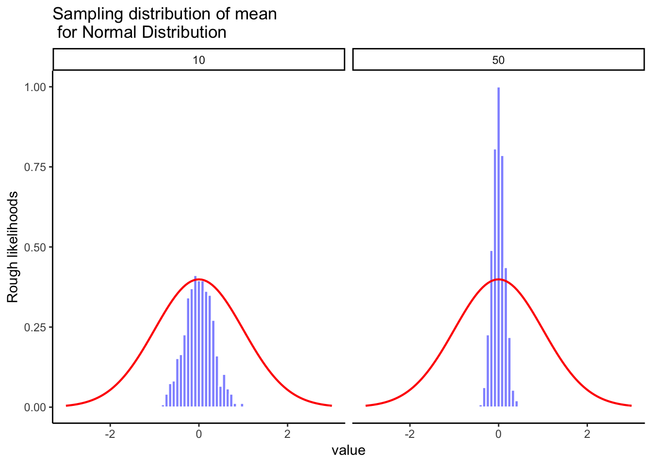
Let's give ourselves a nice movie to see everything in action. We're going to sample numbers from a normal distribution. You will see four panels, each panel represents a different sample size (n), including sample-sizes of 10, 50, 100, and 1000. The red line shows the shape of the normal distribution. The grey bars show a histogram of each of the samples that we take. The red line shows the mean of an individual sample (the middle of the grey bars). As you can see, the red line moves around a lot, especially when the sample size is small (10).

The new bits are the blue bars and the blue lines. The blue bars represent the sampling distribution of the sample mean. For example, in the panel for sample-size 10, we see a bunch of blue bars. This is a histogram of 10 sample means, taken from 10 samples of size 10. In the 50 panel, we see a histogram of 50 sample means, taken from 50 samples of size 50, and so on. The blue line in each panel is the mean of the sample means ("aaagh, it's a mean of means", yes it is).

What should you notice? Notice that the range of the blue bars shrinks as sample size increases. The sampling distribution of the mean is quite wide when the sample-size is 10, it narrows as sample-size increases to 50 and 100, and it's just one bar, right in the middle when sample-size goes to 1000. What we are seeing is that the mean of the sampling distribution approaches the mean of the population as sample-size increases.

So, the sampling distribution of the mean is another distribution, and it has some variance. It varies more when sample-size is small, and varies less when sample-size is large. We can quantify this effect by calculating the standard deviation of the sampling distribution, which is referred to as the standard error. The standard error of a statistic is often denoted SE, and since we're usually interested in the standard error of the sample mean, we often use the acronym SEM. As you can see just by looking at the movie, as the sample size $N$ increases, the SEM decreases.

Okay, so that's one part of the story. However, there's something we've been glossing over a little bit. We've seen it already, but it's worth looking at it one more time. Here's the thing: no matter what shape your population distribution is, as $N$ increases the sampling distribution of the mean starts to look more like a normal distribution. This is the central limit theorem.

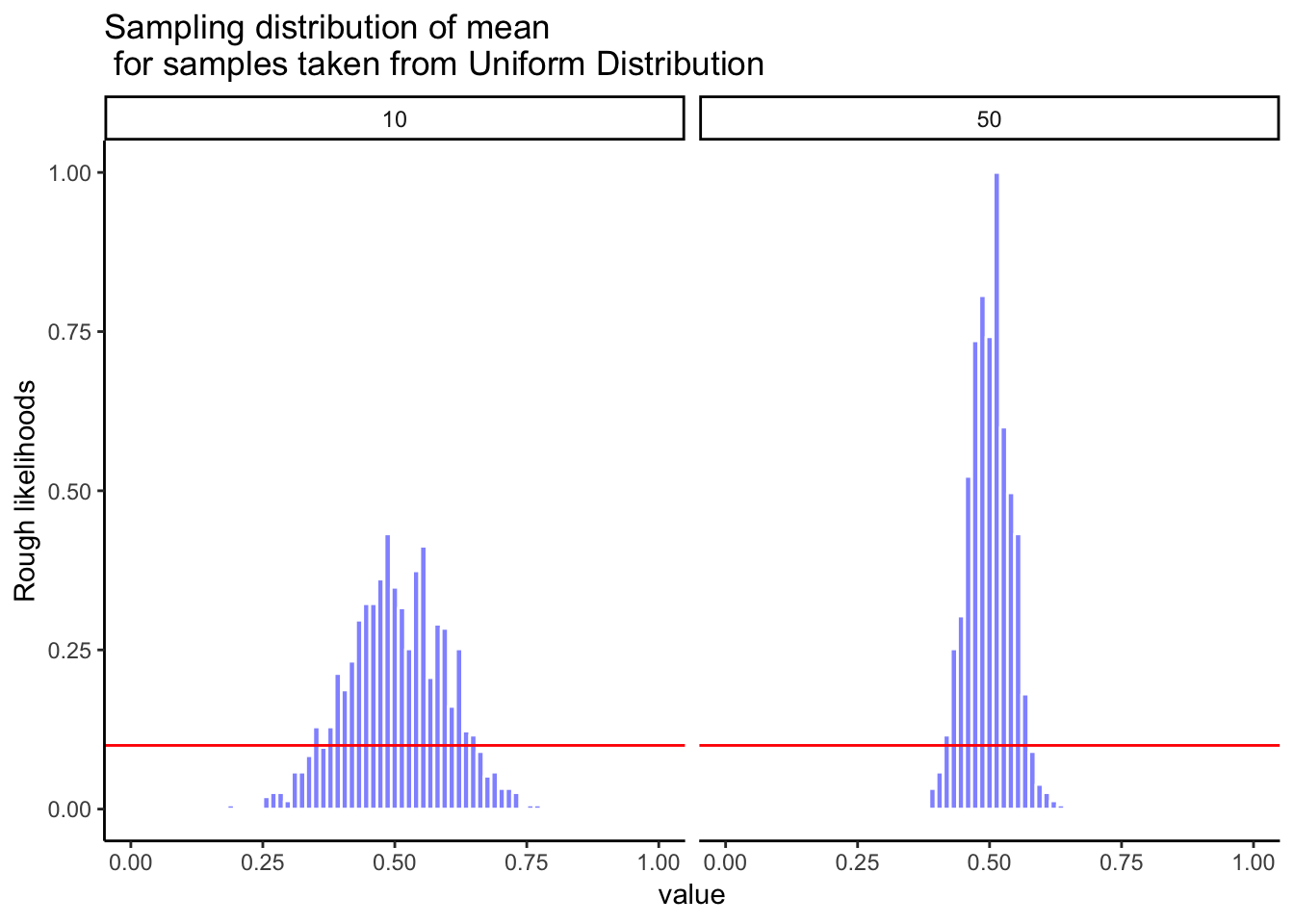
To see the central limit theorem in action, we are going to look at some histograms of sample means different kinds of distributions. It is very important to recognize that you are looking at distributions of sample means, not distributions of individual samples! Here we go, starting with sampling from a normal distribution. The red line is the distribution, the blue bars are the histogram for the sample means. They both look normal!

Let's do it again. This time we sample from a flat uniform distribution. Again, we see that the distribution of the sample means is not flat, it looks like a normal distribution.

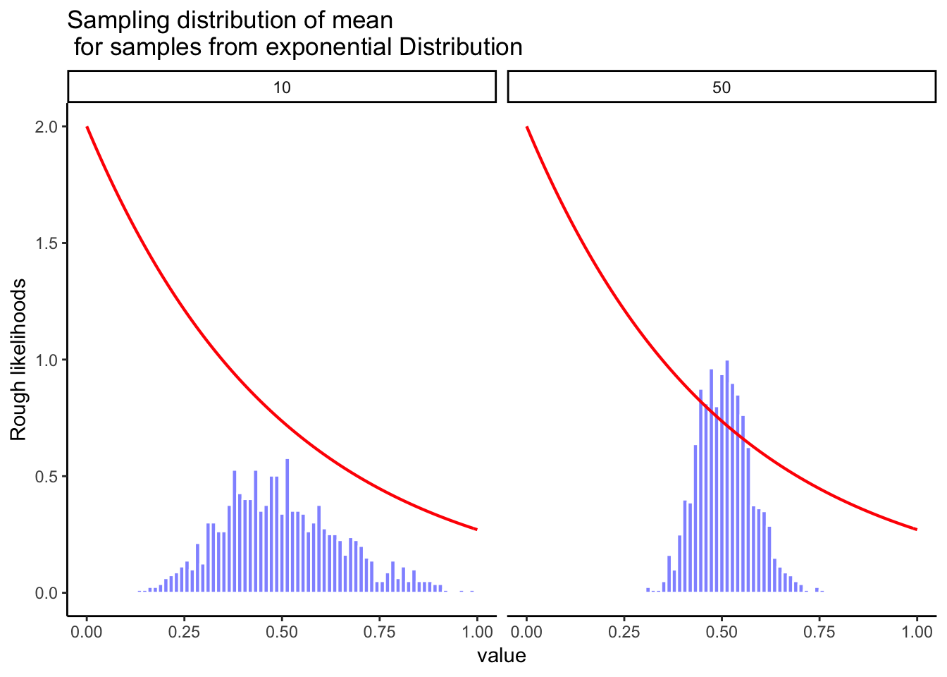
One more time with an exponential distribution. Even though way more of the numbers should be smaller than bigger, then sampling distribution of the mean again does not look the red line. Instead, it looks more normal-ish. That's the central limit theorem. It just works like that.

On the basis of these figures, it seems like we have evidence for all of the following claims about the sampling distribution of the mean:

• The mean of the sampling distribution is the same as the mean of the population

• The standard deviation of the sampling distribution (i.e., the standard error) gets smaller as the sample size increases

• The shape of the sampling distribution becomes normal as the sample size increases

As it happens, not only are all of these statements true, there is a very famous theorem in statistics that proves all three of them, known as the central limit theorem. Among other things, the central limit theorem tells us that if the population distribution has mean $\mu$ and standard deviation $\sigma$, then the sampling distribution of the mean also has mean $\mu$, and the standard error of the mean is $$\mbox{SEM} = \frac{\sigma}{ \sqrt{N} }$$ Because we divide the population standard deviation $\sigma$ by the square root of the sample size $N$, the SEM gets smaller as the sample size increases. It also tells us that the shape of the sampling distribution becomes normal.

This result is useful for all sorts of things. It tells us why large experiments are more reliable than small ones, and because it gives us an explicit formula for the standard error it tells us how much more reliable a large experiment is. It tells us why the normal distribution is, well, normal. In real experiments, many of the things that we want to measure are actually averages of lots of different quantities (e.g., arguably, "general" intelligence as measured by IQ is an average of a large number of "specific" skills and abilities), and when that happens, the averaged quantity should follow a normal distribution. Because of this mathematical law, the normal distribution pops up over and over again in real data.

z-scores

We are now in a position to combine some of things we've been talking about in this chapter, and introduce you to a new tool, z-scores. It turns out we won't use z-scores very much in this textbook. However, you can't take a class on statistics and not learn about z-scores.

The first thing we show you seems to be something that many students remember from their statistics class. This thing is probably remembered because instructors may test this knowledge many times, so students have to learn it for the test. Let's look at this thing. We are going to look at a normal distribution, and we are going to draw lines through the distribution at 0, +/- 1, +/-2, and +/- 3 standard deviations from the mean:

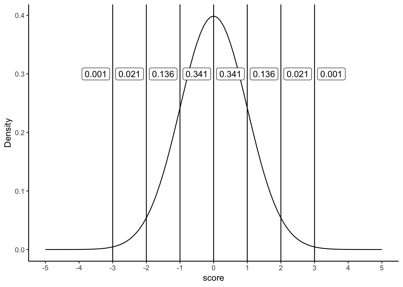
The figure shows a normal distribution with mean = 0, and standard deviation = 1. We've drawn lines at each of the standard deviations: -3, -2, -1, 0, 1, 2, and 3. We also show some numbers in the labels, in between each line. These numbers are proportions. For example, we see the proportion is .341 for scores that fall between the range 0 and 1. Scores between 0 and 1 occur 34.1% of the time. Scores in between -1 and 1, occur 68.2% of the time, that's more than half of the scores. Scores between 1 and occur about 13.6% of the time, and scores between 2 and 3 occur even less, only 2.1% of the time.

Normal distributions always have these properties, even when they have different means and standard deviations. For example, take a look at this normal distribution, it has a mean =100, and standard deviation =25.

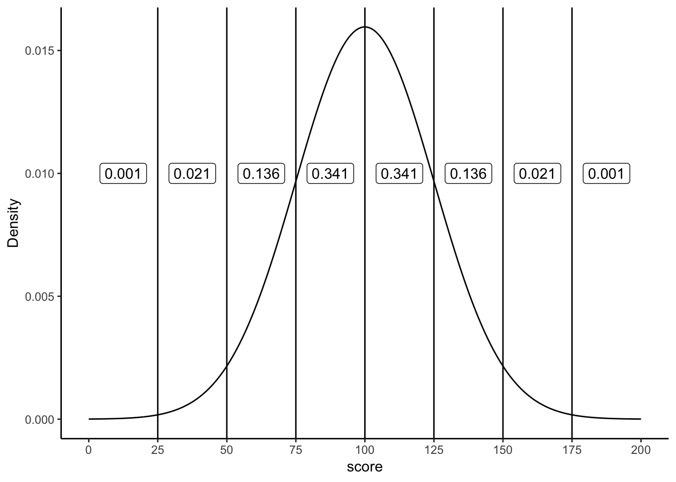
Now we are looking at a normal distribution with mean = 100 and standard deviation = 25. Notice that the region between 100 and 125 contains 34.1% of the scores. This region is 1 standard deviation away from the mean (the standard deviation is 25, the mean is 100, so 25 is one whole standard deviation away from 100). As you can see, the very same proportions occur between each of the standard deviations, as they did when our standard deviation was set to 1 (with a mean of 0).

Idea behind z-scores

Sometimes it can be convenient to transform your original scores into different scores that are easier to work with. For example, if you have a bunch of proportions, like .3, .5, .6, .7, you might want to turn them into percentages like 30%, 50%, 60%, and 70%. To do that you multiply the proportions by a constant of 100. If you want to turn percentages back into proportions, you divide by a constant of 100. This kind of transformation just changes the scale of the numbers from between 0-1, and between 0-100. Otherwise, the pattern in the numbers stays the same.

The idea behind z-scores is a similar kind of transformation. The idea is to express each raw score in terms of it's standard deviation. For example, if I told you I got a 75% on test, you wouldn't know how well I did compared to the rest of the class. But, if I told you that I scored 2 standard deviations above the mean, you'd know I did quite well compared to the rest of the class, because you know that most scores (if they are distributed normally) fall below 2 standard deviations of the mean.

We also know, now thanks to the central limit theorem, that many of our measures, such as sample means, will be distributed normally. So, it can often be desirable to express the raw scores in terms of their standard deviations.

Let's see how this looks in a table without showing you any formulas. We will look at some scores that come from a normal distirbution with mean =100, and standard deviation = 25. We will list some raw scores, along with the z-scores

Remember, the mean is 100, and the standard deviation is 25. How many standard deviations away from the mean is a score of 100? The answer is 0, it's right on the mean. You can see the z-score for 100, is 0. How many standard deviations is 125 away from the mean? Well the standard deviation is 25, 125 is one whole 25 away from 100, that's a total of 1 standard deviation, so the z-score for 125 is 1. The z-score for 150 is 2, because 150 is two 25s away from 100. The z-score for 50 is -2, because 50 is two 25s away from 100 in the opposite direction. All we are doing here is re-expressing the raw scores in terms of how many standard deviations they are from the mean. Remember, the mean is always right on target, so the center of the z-score distribution is always 0.

Calculating z-scores

To calculate z-scores all you have to do is figure out how many standard deviations from the mean each number is. Let's say the mean is 100, and the standard deviation is 25. You have a score of 97. How many standard deviations from the mean is 97?

First compute the difference between the score and the mean:

$97-100 = -3$

Alright, we have a total difference of -3. How many standard deviations does -3 represent if 1 standard deviation is 25? Clearly -3 is much smaller than 25, so it's going to be much less than 1. To figure it out, just divide -3 by the standard deviation.

$\frac{-3}{25} = -.12$

Our z-score for 97 is -.12.

Here's the general formula:

$z = \frac{\text{raw score} - \text{mean}}{\text{standard deviation}}$

So, for example if we had these 10 scores from a normal distribution with mean = 100, and standard deviation =25

The z-scores would be:

Once you have the z-scores, you could use them as another way to describe your data. For example, now just by looking at a score you know if it is likely or unlikely to occur, because you know how the area under the normal curve works. z-scores between -1 and 1 happen pretty often, scores greater than 1 or -1 still happen fairly often, but not as often. And, scores bigger than 2 or -2 don't happen very often. This is a convenient thing to do if you want to look at your numbers and get a general sense of how often they happen.

Usually you do not know the mean or the standard deviation of the population that you are drawing your sample scores from. So, you could use the mean and standard deviation of your sample as an estimate, and then use those to calculate z-scores.

Finally, z-scores are also called standardized scores, because each raw score is described in terms of it's standard deviation. This may well be the last time we talk about z-scores in this book. You might wonder why we even bothered telling you about them. First, it's worth knowing they are a thing. Second, they become important as your statistical prowess becomes more advanced. Third, some statistical concepts, like correlation, can be re-written in terms of z-scores, and this illuminates aspects of those statistics. Finally, they are super useful when you are dealing with a normal distribution that has a known mean and standard deviation.