Dataframes (Pandas) and Plotting (Matplotlib/Seaborn)

Written by Jin Cheong & Luke Chang with modifications and additional by Todd Gureckis

In this lab we are going to learn how to load and manipulate datasets in a dataframe format using Pandas and create beautiful plots using Matplotlib and Seaborn. Pandas is akin to a data frame in R and provides an intuitive way to interact with data in a 2D data frame. Matplotlib is a standard plotting library that is similar in functionality to Matlab's object oriented plotting. Seaborn is also a plotting library built on the Matplotlib framework which carries useful pre-configured plotting schemes.

After the tutorial you will have the chance to apply the methods to a new set of data.

Also, here is a great set of notebooks that also covers the topic. In addition, here is a brief video providing a useful introduction to pandas.

First, we load the basic packages we will be using in this tutorial. Notice how we import the modules using an abbreviated name. This is to reduce the amount of text we type when we use the functions.

Note: %matplotlib inline is an example of 'cell magic' and enables plotting within the notebook and not opening a separate window. In addition, you may want to try using %matplotlib notebook, which will allow more interactive plotting.

%matplotlib inline 

import pandas as pd
import numpy as np
import matplotlib.pyplot as plt
import seaborn as sns

Pandas

Loading Data

We use the pd.read_csv() to load a .csv file into a dataframe. Note that read_csv() has many options that can be used to make sure you load the data correctly.

Pandas has many ways to read data different data formats into a dataframe. Here we will use the pd.read_csv function.

df = pd.read_csv('http://gureckislab.org/courses/fall19/labincp/data/salary.csv', sep = ',', header='infer')

You can always use the ? to access the docstring for a function for more information about the inputs and general useage guidelines.

pd.read_csv?

Ways to check the dataframe

There are many ways to examine your dataframe. One easy way is to execute the dataframe itself.

df
salary gender departm years age publications
0 86285 0 bio 26.0 64.0 72
1 77125 0 bio 28.0 58.0 43
2 71922 0 bio 10.0 38.0 23
3 70499 0 bio 16.0 46.0 64
4 66624 0 bio 11.0 41.0 23
5 64451 0 bio 23.0 60.0 44
6 64366 0 bio 23.0 53.0 22
7 59344 0 bio 5.0 40.0 11
8 58560 0 bio 8.0 38.0 8
9 58294 0 bio 20.0 50.0 12
10 56092 0 bio 2.0 40.0 4
11 54452 0 bio 13.0 43.0 7
12 54269 0 bio 26.0 56.0 12
13 55125 0 bio 8.0 38.0 9
14 97630 0 chem 34.0 64.0 43
15 82444 0 chem 31.0 61.0 42
16 76291 0 chem 29.0 65.0 33
17 75382 0 chem 26.0 56.0 39
18 64762 0 chem 25.0 NaN 29
19 62607 0 chem 20.0 45.0 34
20 60373 0 chem 26.0 56.0 43
21 58892 0 chem 18.0 48.0 21
22 47021 0 chem 4.0 34.0 12
23 44687 0 chem 4.0 34.0 19
24 104828 0 geol NaN 50.0 44
25 71456 0 geol 11.0 41.0 32
26 65144 0 geol 7.0 37.0 12
27 52766 0 geol 4.0 38.0 32
28 112800 0 neuro 14.0 44.0 33
29 105761 0 neuro 9.0 39.0 30
... ... ... ... ... ... ...
47 65285 0 stat 20.0 50.0 15
48 62557 0 stat 28.0 58.0 14
49 61947 0 stat 22.0 58.0 17
50 58565 0 stat 29.0 59.0 11
51 58365 0 stat 18.0 48.0 21
52 53656 0 stat 2.0 32.0 4
53 51391 0 stat 5.0 35.0 8
54 96936 0 physics 15.0 50.0 17
55 83216 0 physics 11.0 37.0 19
56 72044 0 physics 2.0 32.0 16
57 64048 0 physics 23.0 53.0 4
58 58888 0 physics 26.0 56.0 7
59 58744 0 physics 20.0 50.0 9
60 55944 0 physics 21.0 51.0 8
61 54076 0 physics 19.0 49.0 12
62 82142 0 math 9.0 39.0 9
63 70509 0 math 23.0 53.0 7
64 60320 0 math 14.0 44.0 7
65 55814 0 math 8.0 38.0 6
66 53638 0 math 4.0 42.0 8
67 53517 2 math 5.0 35.0 5
68 59139 1 bio 8.0 38.0 23
69 52968 1 bio 18.0 48.0 32
70 55949 1 chem 4.0 34.0 12
71 58893 1 neuro 10.0 35.0 4
72 53662 1 neuro 1.0 31.0 3
73 57185 1 stat 9.0 39.0 7
74 52254 1 stat 2.0 32.0 9
75 61885 1 math 23.0 60.0 9
76 49542 1 math 3.0 33.0 5

77 rows × 6 columns

However, often the dataframes can be large and we may be only interested in seeing the first few rows. df.head() is useful for this purpose. shape is another useful method for getting the dimensions of the matrix. We will print the number of rows and columns in this data set by using output formatting. Use the % sign to indicate the type of data (e.g., %i=integer, %d=float, %s=string), then use the % followed by a tuple of the values you would like to insert into the text. See here for more info about formatting text.

print('There are %i rows and %i columns in this data set' % df.shape) 
There are 77 rows and 6 columns in this data set
df.head()
salary gender departm years age publications
0 86285 0 bio 26.0 64.0 72
1 77125 0 bio 28.0 58.0 43
2 71922 0 bio 10.0 38.0 23
3 70499 0 bio 16.0 46.0 64
4 66624 0 bio 11.0 41.0 23

On the top row, you have column names, that can be called like a dictionary (a dataframe can be essentially thought of as a dictionary with column names as the keys). The left most column (0,1,2,3,4...) is called the index of the dataframe. The default index is sequential integers, but it can be set to anything as long as each row is unique (e.g., subject IDs)

print("Indexes")
print(df.index)
print("Columns")
print(df.columns)
print("Columns are like keys of a dictionary")
print(df.keys())
Indexes
RangeIndex(start=0, stop=77, step=1)
Columns
Index(['salary', 'gender', 'departm', 'years', 'age', 'publications'], dtype='object')
Columns are like keys of a dictionary
Index(['salary', 'gender', 'departm', 'years', 'age', 'publications'], dtype='object')

You can access the values of a column by calling it directly. Double bracket returns a dataframe

df[['salary']]
salary
0 86285
1 77125
2 71922
3 70499
4 66624
5 64451
6 64366
7 59344
8 58560
9 58294
10 56092
11 54452
12 54269
13 55125
14 97630
15 82444
16 76291
17 75382
18 64762
19 62607
20 60373
21 58892
22 47021
23 44687
24 104828
25 71456
26 65144
27 52766
28 112800
29 105761
... ...
47 65285
48 62557
49 61947
50 58565
51 58365
52 53656
53 51391
54 96936
55 83216
56 72044
57 64048
58 58888
59 58744
60 55944
61 54076
62 82142
63 70509
64 60320
65 55814
66 53638
67 53517
68 59139
69 52968
70 55949
71 58893
72 53662
73 57185
74 52254
75 61885
76 49542

77 rows × 1 columns

Single bracket returns a Series

df['salary']
0      86285
1      77125
2      71922
3      70499
4      66624
5      64451
6      64366
7      59344
8      58560
9      58294
10     56092
11     54452
12     54269
13     55125
14     97630
15     82444
16     76291
17     75382
18     64762
19     62607
20     60373
21     58892
22     47021
23     44687
24    104828
25     71456
26     65144
27     52766
28    112800
29    105761
       ...  
47     65285
48     62557
49     61947
50     58565
51     58365
52     53656
53     51391
54     96936
55     83216
56     72044
57     64048
58     58888
59     58744
60     55944
61     54076
62     82142
63     70509
64     60320
65     55814
66     53638
67     53517
68     59139
69     52968
70     55949
71     58893
72     53662
73     57185
74     52254
75     61885
76     49542
Name: salary, Length: 77, dtype: int64

You can also call a column like an attribute if the column name is a string

df.salary
0      86285
1      77125
2      71922
3      70499
4      66624
5      64451
6      64366
7      59344
8      58560
9      58294
10     56092
11     54452
12     54269
13     55125
14     97630
15     82444
16     76291
17     75382
18     64762
19     62607
20     60373
21     58892
22     47021
23     44687
24    104828
25     71456
26     65144
27     52766
28    112800
29    105761
       ...  
47     65285
48     62557
49     61947
50     58565
51     58365
52     53656
53     51391
54     96936
55     83216
56     72044
57     64048
58     58888
59     58744
60     55944
61     54076
62     82142
63     70509
64     60320
65     55814
66     53638
67     53517
68     59139
69     52968
70     55949
71     58893
72     53662
73     57185
74     52254
75     61885
76     49542
Name: salary, Length: 77, dtype: int64

You can create new columns to fit your needs. For instance you can set initialize a new column with zeros.

df['pubperyear'] = 0

Here we can create a new column pubperyear, which is the ratio of the number of papers published per year

df['pubperyear'] = df['publications']/df['years']
df.head()
salary gender departm years age publications pubperyear
0 86285 0 bio 26.0 64.0 72 2.769231
1 77125 0 bio 28.0 58.0 43 1.535714
2 71922 0 bio 10.0 38.0 23 2.300000
3 70499 0 bio 16.0 46.0 64 4.000000
4 66624 0 bio 11.0 41.0 23 2.090909

Indexing and slicing

Indexing in Pandas can be tricky. There are four ways to index: loc, iloc, and explicit indexing(useful for booleans).

First, we will try using .loc. This method references the explicit index. it works for both index names and also column names.

df.loc[0, ['salary']]
salary    86285
Name: 0, dtype: object

Next we wil try .iloc. This method references the implicit python index (starting from 0, exclusive of last number). You can think of this like row by column indexing using integers.

df.iloc[0:3, 0:3]
salary gender departm
0 86285 0 bio
1 77125 0 bio
2 71922 0 bio

Let's make a new data frame with just Males and another for just Females. Notice, how we added the .reset_index(drop=True) method? This is because assigning a new dataframe based on indexing another dataframe will retain the original index. We need to explicitly tell pandas to reset the index if we want it to start from zero.

male_df = df[df.gender == 0].reset_index(drop=True)
female_df = df[df.gender == 1].reset_index(drop=True)

Boolean or logical indexing is useful if you need to sort the data based on some True or False value.

For instance, who are the people with salaries greater than 90K but lower than 100K ?

df[ (df.salary > 90000) & (df.salary < 100000)]
salary gender departm years age publications pubperyear
14 97630 0 chem 34.0 64.0 43 1.264706
30 92951 0 neuro 11.0 41.0 20 1.818182
54 96936 0 physics 15.0 50.0 17 1.133333

Dealing with missing values

It is easy to quickly count the number of missing values for each column in the dataset using the isnull() method. One thing that is nice about Python is that you can chain commands, which means that the output of one method can be the input into the next method. This allows us to write intuitive and concise code. Notice how we take the sum() of all of the null cases.

The isnull() method will return a dataframe with True/False values on whether a datapoint is null or not a number (nan).

df.isnull()
salary gender departm years age publications pubperyear
0 False False False False False False False
1 False False False False False False False
2 False False False False False False False
3 False False False False False False False
4 False False False False False False False
5 False False False False False False False
6 False False False False False False False
7 False False False False False False False
8 False False False False False False False
9 False False False False False False False
10 False False False False False False False
11 False False False False False False False
12 False False False False False False False
13 False False False False False False False
14 False False False False False False False
15 False False False False False False False
16 False False False False False False False
17 False False False False False False False
18 False False False False True False False
19 False False False False False False False
20 False False False False False False False
21 False False False False False False False
22 False False False False False False False
23 False False False False False False False
24 False False False True False False True
25 False False False False False False False
26 False False False False False False False
27 False False False False False False False
28 False False False False False False False
29 False False False False False False False
... ... ... ... ... ... ... ...
47 False False False False False False False
48 False False False False False False False
49 False False False False False False False
50 False False False False False False False
51 False False False False False False False
52 False False False False False False False
53 False False False False False False False
54 False False False False False False False
55 False False False False False False False
56 False False False False False False False
57 False False False False False False False
58 False False False False False False False
59 False False False False False False False
60 False False False False False False False
61 False False False False False False False
62 False False False False False False False
63 False False False False False False False
64 False False False False False False False
65 False False False False False False False
66 False False False False False False False
67 False False False False False False False
68 False False False False False False False
69 False False False False False False False
70 False False False False False False False
71 False False False False False False False
72 False False False False False False False
73 False False False False False False False
74 False False False False False False False
75 False False False False False False False
76 False False False False False False False

77 rows × 7 columns

We can chain the .null() and .sum() methods to see how many null values are added up.

df.isnull().sum()
salary          0
gender          0
departm         0
years           1
age             1
publications    0
pubperyear      1
dtype: int64

You can use the boolean indexing once again to see the datapoints that have missing values. We chained the method .any() which will check if there are any True values for a given axis. Axis=0 indicates rows, while Axis=1 indicates columns. So here we are creating a boolean index for row where any column has a missing value.

df[df.isnull().any(axis=1)]
salary gender departm years age publications pubperyear
18 64762 0 chem 25.0 NaN 29 1.16
24 104828 0 geol NaN 50.0 44 NaN

You may look at where the values are not null. Note that indexes 18, and 24 are missing.

df[~df.isnull().any(axis=1)]
salary gender departm years age publications pubperyear salary_in_departm dept_num
0 86285 0 bio 26.0 64.0 72 2.769231 2.468065 0
1 77125 0 bio 28.0 58.0 43 1.535714 1.493198 0
2 71922 0 bio 10.0 38.0 23 2.300000 0.939461 0
3 70499 0 bio 16.0 46.0 64 4.000000 0.788016 0
4 66624 0 bio 11.0 41.0 23 2.090909 0.375613 0
5 64451 0 bio 23.0 60.0 44 1.913043 0.144348 0
6 64366 0 bio 23.0 53.0 22 0.956522 0.135301 0
7 59344 0 bio 5.0 40.0 11 2.200000 -0.399173 0
8 58560 0 bio 8.0 38.0 8 1.000000 -0.482611 0
9 58294 0 bio 20.0 50.0 12 0.600000 -0.510921 0
10 56092 0 bio 2.0 40.0 4 2.000000 -0.745272 0
11 54452 0 bio 13.0 43.0 7 0.538462 -0.919812 0
12 54269 0 bio 26.0 56.0 12 0.461538 -0.939288 0
13 55125 0 bio 8.0 38.0 9 1.125000 -0.848186 0
14 97630 0 chem 34.0 64.0 43 1.264706 1.900129 1
15 82444 0 chem 31.0 61.0 42 1.354839 0.984156 1
16 76291 0 chem 29.0 65.0 33 1.137931 0.613025 1
17 75382 0 chem 26.0 56.0 39 1.500000 0.558197 1
19 62607 0 chem 20.0 45.0 34 1.700000 -0.212352 1
20 60373 0 chem 26.0 56.0 43 1.653846 -0.347100 1
21 58892 0 chem 18.0 48.0 21 1.166667 -0.436429 1
22 47021 0 chem 4.0 34.0 12 3.000000 -1.152452 1
23 44687 0 chem 4.0 34.0 19 4.750000 -1.293232 1
25 71456 0 geol 11.0 41.0 32 2.909091 0.876557 2
26 65144 0 geol 7.0 37.0 12 1.714286 0.212671 2
27 52766 0 geol 4.0 38.0 32 8.000000 -1.089228 2
28 112800 0 neuro 14.0 44.0 33 2.357143 2.024705 3
29 105761 0 neuro 9.0 39.0 30 3.333333 1.632462 3
30 92951 0 neuro 11.0 41.0 20 1.818182 0.918635 3
31 86621 0 neuro 19.0 49.0 10 0.526316 0.565901 3
... ... ... ... ... ... ... ... ... ...
46 69596 0 stat 20.0 50.0 18 0.900000 0.158420 4
47 65285 0 stat 20.0 50.0 15 0.750000 -0.131801 4
48 62557 0 stat 28.0 58.0 14 0.500000 -0.315453 4
49 61947 0 stat 22.0 58.0 17 0.772727 -0.356519 4
50 58565 0 stat 29.0 59.0 11 0.379310 -0.584199 4
51 58365 0 stat 18.0 48.0 21 1.166667 -0.597664 4
52 53656 0 stat 2.0 32.0 4 2.000000 -0.914679 4
53 51391 0 stat 5.0 35.0 8 1.600000 -1.067161 4
54 96936 0 physics 15.0 50.0 17 1.133333 1.909602 5
55 83216 0 physics 11.0 37.0 19 1.727273 1.004571 5
56 72044 0 physics 2.0 32.0 16 8.000000 0.267617 5
57 64048 0 physics 23.0 53.0 4 0.173913 -0.259834 5
58 58888 0 physics 26.0 56.0 7 0.269231 -0.600210 5
59 58744 0 physics 20.0 50.0 9 0.450000 -0.609708 5
60 55944 0 physics 21.0 51.0 8 0.380952 -0.794409 5
61 54076 0 physics 19.0 49.0 12 0.631579 -0.917630 5
62 82142 0 math 9.0 39.0 9 1.000000 1.810331 6
63 70509 0 math 23.0 53.0 7 0.304348 0.765887 6
64 60320 0 math 14.0 44.0 7 0.500000 -0.148911 6
65 55814 0 math 8.0 38.0 6 0.750000 -0.553473 6
66 53638 0 math 4.0 42.0 8 2.000000 -0.748841 6
68 59139 1 bio 8.0 38.0 23 2.875000 -0.420990 0
69 52968 1 bio 18.0 48.0 32 1.777778 -1.077749 0
70 55949 1 chem 4.0 34.0 12 3.000000 -0.613942 1
71 58893 1 neuro 10.0 35.0 4 0.400000 -0.979219 3
72 53662 1 neuro 1.0 31.0 3 3.000000 -1.270712 3
73 57185 1 stat 9.0 39.0 7 0.777778 -0.677103 4
74 52254 1 stat 2.0 32.0 9 4.500000 -1.009063 4
75 61885 1 math 23.0 60.0 9 0.391304 -0.008401 6
76 49542 1 math 3.0 33.0 5 1.666667 -1.116592 6

74 rows × 9 columns

There are different techniques for dealing with missing data. An easy one is to simply remove rows that have any missing values using the dropna() method.

df = df.dropna()

Now we can check to make sure the missing rows are removed. Let's also check the new dimensions of the dataframe.

print('There are %i rows and %i columns in this data set' % df.shape)
df.isnull().sum()
There are 75 rows and 7 columns in this data set
salary          0
gender          0
departm         0
years           0
age             0
publications    0
pubperyear      0
dtype: int64

Describing the data

We can use the .describe() method to get a quick summary of the continuous values of the data frame. We will .transpose() the output to make it slightly easier to read.

df.describe().transpose()
count mean std min 25% 50% 75% max
salary 75.0 67293.946667 14672.455177 44687.000000 56638.500000 62557.000000 74733.500000 112800.0
gender 75.0 0.146667 0.392268 0.000000 0.000000 0.000000 0.000000 2.0
years 75.0 14.840000 8.596102 1.000000 8.000000 14.000000 22.500000 34.0
age 75.0 45.426667 9.051166 31.000000 38.000000 44.000000 53.000000 65.0
publications 75.0 21.440000 15.200676 3.000000 9.000000 18.000000 32.500000 72.0
pubperyear 75.0 1.926595 1.602968 0.173913 0.775253 1.653846 2.563187 8.0

We can also get quick summary of a pandas series, or specific column of a pandas dataframe.

df.departm.describe()
count      75
unique      7
top       bio
freq       16
Name: departm, dtype: object

Manipulating data in Groups

One manipulation we often do is look at variables in groups. One way to do this is to usethe .groupby(key) method. The key is a column that is used to group the variables together. For instance, if we want to group the data by gender and get group means, we perform the following.

df.groupby('gender').mean()
salary years age publications pubperyear
gender
0 69108.492308 15.846154 46.492308 23.061538 1.924709
1 55719.666667 8.666667 38.888889 11.555556 2.043170
2 53517.000000 5.000000 35.000000 5.000000 1.000000

Other default aggregation methods include .count(), .mean(), .median(), .min(), .max(), .std(), .var(), and .sum()

Before we move on, it looks like there were more than 2 genders specified in our data. This is likely an error in the data collection process so let recap on how we might remove this datapoint.

df[df['gender']==2]
salary gender departm years age publications pubperyear
67 53517 2 math 5.0 35.0 5 1.0

replace original dataframe without the miscoded data

df = df[df['gender']!=2]

Now we have a corrected dataframe!

df.groupby('gender').mean()
salary years age publications pubperyear
gender
0 69108.492308 15.846154 46.492308 23.061538 1.924709
1 55719.666667 8.666667 38.888889 11.555556 2.043170

Another powerful tool in Pandas is the split-apply-combine method. For instance, let's say we also want to look at how much each professor is earning in respect to the department. Let's say we want to subtract the departmental mean from professor and divide it by the departmental standard deviation. We can do this by using the groupby(key) method chained with the .transform(function) method. It will group the dataframe by the key column, perform the "function" transformation of the data and return data in same format. To learn more, see link here

# key: We use the departm as the grouping factor. 
key = df['departm']

# Let's create an anonmyous function for calculating zscores using lambda:
# We want to standardize salary for each department.
zscore = lambda x: (x - x.mean()) / x.std()

# Now let's calculate zscores separately within each department
transformed = df.groupby(key).transform(zscore)
df['salary_in_departm'] = transformed['salary']

Now we have salary_in_departm column showing standardized salary per department.

df.head()
salary gender departm years age publications pubperyear salary_in_departm
0 86285 0 bio 26.0 64.0 72 2.769231 2.468065
1 77125 0 bio 28.0 58.0 43 1.535714 1.493198
2 71922 0 bio 10.0 38.0 23 2.300000 0.939461
3 70499 0 bio 16.0 46.0 64 4.000000 0.788016
4 66624 0 bio 11.0 41.0 23 2.090909 0.375613

Combining datasets - pd.concat

Recall that we sliced the dataframes into male and female dataframe in 2.3 Indexing and Slicing. Now we will learn how to put dataframes together which is done by the pd.concat method. Note how the index of this output retains the old index.

pd.concat([femaledf, maledf],axis = 0)
salary gender departm years age publications pubperyear
0 59139 1 bio 8.0 38.0 23 2.875000
1 52968 1 bio 18.0 48.0 32 1.777778
2 55949 1 chem 4.0 34.0 12 3.000000
3 58893 1 neuro 10.0 35.0 4 0.400000
4 53662 1 neuro 1.0 31.0 3 3.000000
5 57185 1 stat 9.0 39.0 7 0.777778
6 52254 1 stat 2.0 32.0 9 4.500000
7 61885 1 math 23.0 60.0 9 0.391304
8 49542 1 math 3.0 33.0 5 1.666667
0 86285 0 bio 26.0 64.0 72 2.769231
1 77125 0 bio 28.0 58.0 43 1.535714
2 71922 0 bio 10.0 38.0 23 2.300000
3 70499 0 bio 16.0 46.0 64 4.000000
4 66624 0 bio 11.0 41.0 23 2.090909
5 64451 0 bio 23.0 60.0 44 1.913043
6 64366 0 bio 23.0 53.0 22 0.956522
7 59344 0 bio 5.0 40.0 11 2.200000
8 58560 0 bio 8.0 38.0 8 1.000000
9 58294 0 bio 20.0 50.0 12 0.600000
10 56092 0 bio 2.0 40.0 4 2.000000
11 54452 0 bio 13.0 43.0 7 0.538462
12 54269 0 bio 26.0 56.0 12 0.461538
13 55125 0 bio 8.0 38.0 9 1.125000
14 97630 0 chem 34.0 64.0 43 1.264706
15 82444 0 chem 31.0 61.0 42 1.354839
16 76291 0 chem 29.0 65.0 33 1.137931
17 75382 0 chem 26.0 56.0 39 1.500000
18 64762 0 chem 25.0 NaN 29 1.160000
19 62607 0 chem 20.0 45.0 34 1.700000
20 60373 0 chem 26.0 56.0 43 1.653846
... ... ... ... ... ... ... ...
37 66482 0 neuro 14.0 44.0 42 3.000000
38 61680 0 neuro 18.0 48.0 20 1.111111
39 60455 0 neuro 8.0 38.0 49 6.125000
40 58932 0 neuro 11.0 41.0 49 4.454545
41 106412 0 stat 23.0 53.0 29 1.260870
42 86980 0 stat 23.0 53.0 42 1.826087
43 78114 0 stat 8.0 38.0 24 3.000000
44 74085 0 stat 11.0 41.0 33 3.000000
45 72250 0 stat 26.0 56.0 9 0.346154
46 69596 0 stat 20.0 50.0 18 0.900000
47 65285 0 stat 20.0 50.0 15 0.750000
48 62557 0 stat 28.0 58.0 14 0.500000
49 61947 0 stat 22.0 58.0 17 0.772727
50 58565 0 stat 29.0 59.0 11 0.379310
51 58365 0 stat 18.0 48.0 21 1.166667
52 53656 0 stat 2.0 32.0 4 2.000000
53 51391 0 stat 5.0 35.0 8 1.600000
54 96936 0 physics 15.0 50.0 17 1.133333
55 83216 0 physics 11.0 37.0 19 1.727273
56 72044 0 physics 2.0 32.0 16 8.000000
57 64048 0 physics 23.0 53.0 4 0.173913
58 58888 0 physics 26.0 56.0 7 0.269231
59 58744 0 physics 20.0 50.0 9 0.450000
60 55944 0 physics 21.0 51.0 8 0.380952
61 54076 0 physics 19.0 49.0 12 0.631579
62 82142 0 math 9.0 39.0 9 1.000000
63 70509 0 math 23.0 53.0 7 0.304348
64 60320 0 math 14.0 44.0 7 0.500000
65 55814 0 math 8.0 38.0 6 0.750000
66 53638 0 math 4.0 42.0 8 2.000000

76 rows × 7 columns

We can reset the index to start at zero using the .reset_index() method

pd.concat([maledf, femaledf], axis = 0).reset_index(drop=True)
salary gender departm years age publications pubperyear
0 86285 0 bio 26.0 64.0 72 2.769231
1 77125 0 bio 28.0 58.0 43 1.535714
2 71922 0 bio 10.0 38.0 23 2.300000
3 70499 0 bio 16.0 46.0 64 4.000000
4 66624 0 bio 11.0 41.0 23 2.090909
5 64451 0 bio 23.0 60.0 44 1.913043
6 64366 0 bio 23.0 53.0 22 0.956522
7 59344 0 bio 5.0 40.0 11 2.200000
8 58560 0 bio 8.0 38.0 8 1.000000
9 58294 0 bio 20.0 50.0 12 0.600000
10 56092 0 bio 2.0 40.0 4 2.000000
11 54452 0 bio 13.0 43.0 7 0.538462
12 54269 0 bio 26.0 56.0 12 0.461538
13 55125 0 bio 8.0 38.0 9 1.125000
14 97630 0 chem 34.0 64.0 43 1.264706
15 82444 0 chem 31.0 61.0 42 1.354839
16 76291 0 chem 29.0 65.0 33 1.137931
17 75382 0 chem 26.0 56.0 39 1.500000
18 64762 0 chem 25.0 NaN 29 1.160000
19 62607 0 chem 20.0 45.0 34 1.700000
20 60373 0 chem 26.0 56.0 43 1.653846
21 58892 0 chem 18.0 48.0 21 1.166667
22 47021 0 chem 4.0 34.0 12 3.000000
23 44687 0 chem 4.0 34.0 19 4.750000
24 104828 0 geol NaN 50.0 44 NaN
25 71456 0 geol 11.0 41.0 32 2.909091
26 65144 0 geol 7.0 37.0 12 1.714286
27 52766 0 geol 4.0 38.0 32 8.000000
28 112800 0 neuro 14.0 44.0 33 2.357143
29 105761 0 neuro 9.0 39.0 30 3.333333
... ... ... ... ... ... ... ...
46 69596 0 stat 20.0 50.0 18 0.900000
47 65285 0 stat 20.0 50.0 15 0.750000
48 62557 0 stat 28.0 58.0 14 0.500000
49 61947 0 stat 22.0 58.0 17 0.772727
50 58565 0 stat 29.0 59.0 11 0.379310
51 58365 0 stat 18.0 48.0 21 1.166667
52 53656 0 stat 2.0 32.0 4 2.000000
53 51391 0 stat 5.0 35.0 8 1.600000
54 96936 0 physics 15.0 50.0 17 1.133333
55 83216 0 physics 11.0 37.0 19 1.727273
56 72044 0 physics 2.0 32.0 16 8.000000
57 64048 0 physics 23.0 53.0 4 0.173913
58 58888 0 physics 26.0 56.0 7 0.269231
59 58744 0 physics 20.0 50.0 9 0.450000
60 55944 0 physics 21.0 51.0 8 0.380952
61 54076 0 physics 19.0 49.0 12 0.631579
62 82142 0 math 9.0 39.0 9 1.000000
63 70509 0 math 23.0 53.0 7 0.304348
64 60320 0 math 14.0 44.0 7 0.500000
65 55814 0 math 8.0 38.0 6 0.750000
66 53638 0 math 4.0 42.0 8 2.000000
67 59139 1 bio 8.0 38.0 23 2.875000
68 52968 1 bio 18.0 48.0 32 1.777778
69 55949 1 chem 4.0 34.0 12 3.000000
70 58893 1 neuro 10.0 35.0 4 0.400000
71 53662 1 neuro 1.0 31.0 3 3.000000
72 57185 1 stat 9.0 39.0 7 0.777778
73 52254 1 stat 2.0 32.0 9 4.500000
74 61885 1 math 23.0 60.0 9 0.391304
75 49542 1 math 3.0 33.0 5 1.666667

76 rows × 7 columns

Plotting in pandas

Before we move into Matplotlib, here are a few plotting methods already implemented in Pandas.

Boxplot

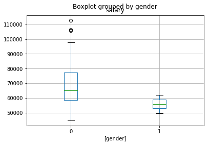
df[['salary','gender']].boxplot(by='gender')
<matplotlib.axes._subplots.AxesSubplot at 0x1a1d97f320>

Scatterplot

df[['salary', 'years']].plot(kind='scatter', x='years', y='salary')
<matplotlib.axes._subplots.AxesSubplot at 0x1a1dc9df28>

Plotting Categorical Variables. Replacing variables with .map

If we want to plot department on the x-axis, Pandas plotting functions won't know what to do because they don't know where to put bio or chem on a numerical x-axis. Therefore one needs to change them to numerical variable to plot them with basic functionalities (we will later see how Seaborn sovles this).

df['dept_num'] = 0
df.loc[:, ['dept_num']] = df.departm.map({'bio':0, 'chem':1, 'geol':2, 'neuro':3, 'stat':4, 'physics':5, 'math':6})
df.tail()
salary gender departm years age publications pubperyear salary_in_departm dept_num
72 53662 1 neuro 1.0 31.0 3 3.000000 -1.270712 3
73 57185 1 stat 9.0 39.0 7 0.777778 -0.677103 4
74 52254 1 stat 2.0 32.0 9 4.500000 -1.009063 4
75 61885 1 math 23.0 60.0 9 0.391304 -0.008401 6
76 49542 1 math 3.0 33.0 5 1.666667 -1.116592 6

Now plot all four categories

f, axs = plt.subplots(1, 4, sharey=True)
f.suptitle('Salary in relation to other variables')
df.plot(kind='scatter', x='gender', y='salary', ax=axs[0], figsize=(15, 4))
df.plot(kind='scatter', x='dept_num', y='salary', ax=axs[1])
df.plot(kind='scatter', x='years', y='salary', ax=axs[2])
df.plot(kind='scatter', x='age', y='salary', ax=axs[3])
<matplotlib.axes._subplots.AxesSubplot at 0x1a1dedb128>

The problem is that it treats department as a continuous variable.

Generating bar - errorbar plots in Pandas

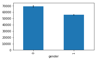
means = df.groupby('gender').mean()['salary']
errors = df.groupby('gender').std()['salary'] / np.sqrt(df.groupby('gender').count()['salary'])
ax = means.plot.bar(yerr=errors,figsize=(5,3))

Matplotlib

Matplotlib is an object oriented plotting library in Python that is loosely based off of plotting in matlab. It is the primary library that many other packages build on. Here is a very concise and helpful introduction to plotting in Python. Learn other matplotlib tutorials here

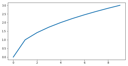
create a basic lineplot

plt.figure(figsize=(8, 4))
plt.plot(range(0, 10),np.sqrt(range(0,10)), linewidth=3)
[<matplotlib.lines.Line2D at 0x1a1ee93630>]

create a basic scatterplot

plt.figure(figsize=(4, 4))
plt.scatter(df.salary, df.age, color='b', marker='*')
<matplotlib.collections.PathCollection at 0x1a1ee3e2b0>

Modify different aspects of the plot

subplots allows you to control different aspects of multiple plots

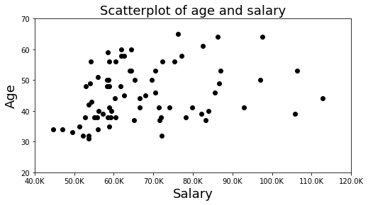
f,ax = plt.subplots(nrows=1, ncols=1, figsize=(8, 4)) 
ax.scatter(df.salary, df.age,color='k', marker='o')
ax.set_xlim([40000,120000])
ax.set_ylim([20,70])
ax.set_xticklabels([str(int(tick)/1000)+'K' for tick in ax.get_xticks()])
ax.set_xlabel('Salary', fontsize=18)
ax.set_ylabel('Age', fontsize=18)
ax.set_title('Scatterplot of age and salary', fontsize=18)
Text(0.5, 1.0, 'Scatterplot of age and salary')

We can save the plot using the savefig command.

f.savefig('MyFirstPlot.png')

Create multiple plots

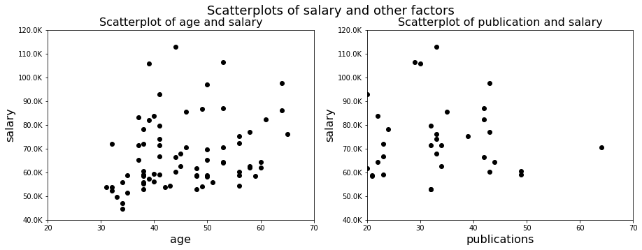
f,axs = plt.subplots(1, 2, figsize=(15,5)) 
axs[0].scatter(df.age, df.salary, color='k', marker='o')
axs[0].set_ylim([40000, 120000])
axs[0].set_xlim([20, 70])
axs[0].set_yticklabels([str(int(tick)/1000)+'K' for tick in axs[0].get_yticks()])
axs[0].set_ylabel('salary', fontsize=16)
axs[0].set_xlabel('age', fontsize=16)
axs[0].set_title('Scatterplot of age and salary', fontsize=16)

axs[1].scatter(df.publications, df.salary,color='k',marker='o')
axs[1].set_ylim([40000, 120000])
axs[1].set_xlim([20, 70])
axs[1].set_yticklabels([str(int(tick)/1000)+'K' for tick in axs[1].get_yticks()])

axs[1].set_ylabel('salary', fontsize=16)
axs[1].set_xlabel('publications', fontsize=16)
axs[1].set_title('Scatterplot of publication and salary', fontsize=16)

f.suptitle('Scatterplots of salary and other factors', fontsize=18)
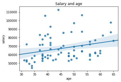
Text(0.5, 0.98, 'Scatterplots of salary and other factors')

Seaborn

Seaborn is a plotting library built on Matplotlib that has many pre-configured plots that are often used for visualization. Other great tutorials about seaborn are here

ax = sns.regplot(df.age, df.salary)
ax.set_title('Salary and age')
Text(0.5, 1.0, 'Salary and age')
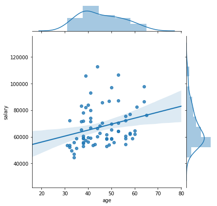
sns.jointplot("age", "salary", data=df, kind='reg')
<seaborn.axisgrid.JointGrid at 0x1a1f0ebb00>

Factor plots

Factor plots allow you to visualize the distribution of parameters in different forms such as point, bar, or violin graphs.

Here are some possible values for kind : {point, bar, count, box, violin, strip}

sns.catplot(x='departm', y='salary', hue='gender', data=df, ci=68, kind='bar')
<seaborn.axisgrid.FacetGrid at 0x1a1e49bc18>

Heatmap plots

Heatmap plots allow you to visualize matrices such as correlation matrices that show relationships across multiple variables

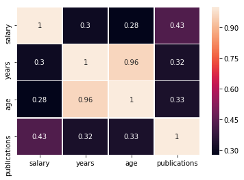
sns.heatmap(df[['salary', 'years', 'age', 'publications']].corr(), annot=True, linewidths=.5)
<matplotlib.axes._subplots.AxesSubplot at 0x1a1fc82828>